第 4 章 词间关系:n元组(n-grams)及相关度
到此为止,我们一直把词看作独立的单元,并考量词与情感或与文档间的关系。然而,很多有意思的文本分析基于词间关系,无论是考察哪个词更经常紧跟另外的词,或是更趋向同时出现在同一文档中的词。
本章中,我们将探索 tidytext 提供的一些方法,计算和绘制文本数据集中词与词之间的关系。包括 token = "ngrams" 参数,按照邻接的词对进行符号化而非按单个词。我们还将介绍两个新的包:ggraph (Pedersen 2021),扩展 ggplot2 以创建网络点图,以及 widyr (Robinson 2020b),可按词对计算相关及在 tidy 数据框中计算距离。这将扩充我们探索 tidy 数据框架的的工具箱。
4.1 按n元组符号化
We’ve been using the unnest_tokens function to tokenize by word, or sometimes by sentence, which is useful for the kinds of sentiment and frequency analyses we’ve been doing so far. But we can also use the function to tokenize into consecutive sequences of words, called n-grams. By seeing how often word X is followed by word Y, we can then build a model of the relationships between them.
We do this by adding the token = "ngrams" option to unnest_tokens(), and setting n to the number of words we wish to capture in each n-gram. When we set n to 2, we are examining pairs of two consecutive words, often called “bigrams”:
library(gutenbergr)

hongloumeng_en <- gutenberg_download(c(9603, 9604), meta_fields = "title")library(dplyr)
library(tidytext)
library(stringr)
bigrams <- hongloumeng_en %>%
mutate(book = cumsum(str_detect(text, regex("HUNG LOU MENG, BOOK [I]+")))) %>%
unnest_tokens(bigram, text, token = "ngrams", n = 2)
bigrams## # A tibble: 420,779 x 4
## gutenberg_id title book bigram
## <int> <chr> <int> <chr>
## 1 9603 Hung Lou Meng, or, the Dream of the Red Chamber, a Chinese Novel, Bo~ 1 hung lou
## 2 9603 Hung Lou Meng, or, the Dream of the Red Chamber, a Chinese Novel, Bo~ 1 lou meng
## 3 9603 Hung Lou Meng, or, the Dream of the Red Chamber, a Chinese Novel, Bo~ 1 meng bo~
## 4 9603 Hung Lou Meng, or, the Dream of the Red Chamber, a Chinese Novel, Bo~ 1 book i
## 5 9603 Hung Lou Meng, or, the Dream of the Red Chamber, a Chinese Novel, Bo~ 1 <NA>
## 6 9603 Hung Lou Meng, or, the Dream of the Red Chamber, a Chinese Novel, Bo~ 1 or the
## 7 9603 Hung Lou Meng, or, the Dream of the Red Chamber, a Chinese Novel, Bo~ 1 the dre~
## 8 9603 Hung Lou Meng, or, the Dream of the Red Chamber, a Chinese Novel, Bo~ 1 dream of
## 9 9603 Hung Lou Meng, or, the Dream of the Red Chamber, a Chinese Novel, Bo~ 1 of the
## 10 9603 Hung Lou Meng, or, the Dream of the Red Chamber, a Chinese Novel, Bo~ 1 the red
## # ... with 420,769 more rowsThis data structure is still a variation of the tidy text format. It is structured as one-token-per-row (with extra metadata, such as book, still preserved), but each token now represents a bigram.
Notice that these bigrams overlap: “sense and” is one token, while “and sensibility” is another.
4.1.1 计算和过滤n元组
Our usual tidy tools apply equally well to n-gram analysis. We can examine the most common bigrams using dplyr’s count():
bigrams %>%
  count(bigram, sort = TRUE)
## # A tibble: 139,813 x 2
## bigram n
## <chr> <int>
## 1 <NA> 8786
## 2 of the 2342
## 3 pao yue 1936
## 4 in the 1466
## 5 on the 1032
## 6 to the 910
## 7 lady feng 820
## 8 tai yue 672
## 9 and the 648
## 10 lady chia 616
## # ... with 139,803 more rowsAs one might expect, a lot of the most common bigrams are pairs of common (uninteresting) words, such as of the and to be: what we call “stop-words” (see Chapter 1). This is a useful time to use tidyr’s separate(), which splits a column into multiple based on a delimiter. This lets us separate it into two columns, “word1” and “word2,” at which point we can remove cases where either is a stop-word.
library(tidyr)

bigrams_separated <- bigrams %>%
  separate(bigram, c("word1", "word2"), sep = " ")
bigrams_filtered <- bigrams_separated %>%
  filter(!word1 %in% stop_words$word) %>%
  filter(!word2 %in% stop_words$word)
# new bigram counts:
bigram_counts <- bigrams_filtered %>%
  count(word1, word2, sort = TRUE)
bigram_counts
## # A tibble: 25,811 x 3
## word1 word2 n
## <chr> <chr> <int>
## 1 <NA> <NA> 8786
## 2 pao yue 1936
## 3 lady feng 820
## 4 tai yue 672
## 5 lady chia 616
## 6 pao ch'ai 555
## 7 hsi jen 482
## 8 dowager lady 448
## 9 madame wang 390
## 10 p'ing erh 297
## # ... with 25,801 more rowsWe can see that names (whether first and last or with a salutation) are the most common pairs.
In other analyses, we may want to work with the recombined words. tidyr’s unite() function is the inverse of separate(), and lets us recombine the columns into one. Thus, “separate/filter/count/unite” let us find the most common bigrams not containing stop-words.
bigrams_united <- bigrams_filtered %>%
  unite(bigram, word1, word2, sep = " ")
bigrams_united
## # A tibble: 56,075 x 4
## gutenberg_id title book bigram
## <int> <chr> <int> <chr>
## 1 9603 Hung Lou Meng, or, the Dream of the Red Chamber, a Chinese Novel, ~ 1 hung lou
## 2 9603 Hung Lou Meng, or, the Dream of the Red Chamber, a Chinese Novel, ~ 1 lou meng
## 3 9603 Hung Lou Meng, or, the Dream of the Red Chamber, a Chinese Novel, ~ 1 meng book
## 4 9603 Hung Lou Meng, or, the Dream of the Red Chamber, a Chinese Novel, ~ 1 NA NA
## 5 9603 Hung Lou Meng, or, the Dream of the Red Chamber, a Chinese Novel, ~ 1 red chamb~
## 6 9603 Hung Lou Meng, or, the Dream of the Red Chamber, a Chinese Novel, ~ 1 NA NA
## 7 9603 Hung Lou Meng, or, the Dream of the Red Chamber, a Chinese Novel, ~ 1 NA NA
## 8 9603 Hung Lou Meng, or, the Dream of the Red Chamber, a Chinese Novel, ~ 1 NA NA
## 9 9603 Hung Lou Meng, or, the Dream of the Red Chamber, a Chinese Novel, ~ 1 cao xueqin
## 10 9603 Hung Lou Meng, or, the Dream of the Red Chamber, a Chinese Novel, ~ 1 NA NA
## # ... with 56,065 more rowsIn other analyses you may be interested in the most common trigrams, which are consecutive sequences of 3 words. We can find this by setting n = 3:
hongloumeng_en %>%
  unnest_tokens(trigram, text, token = "ngrams", n = 3) %>%
  separate(trigram, c("word1", "word2", "word3"), sep = " ") %>%
  filter(!word1 %in% stop_words$word,
         !word2 %in% stop_words$word,
         !word3 %in% stop_words$word) %>%
  count(word1, word2, word3, sort = TRUE)
## # A tibble: 12,509 x 4
## word1 word2 word3 n
## <chr> <chr> <chr> <int>
## 1 <NA> <NA> <NA> 9427
## 2 dowager lady chia 362
## 3 lin tai yue 159
## 4 shih hsiang yuen 60
## 5 chou jui's wife 58
## 6 dowager lady chia's 45
## 7 pao yue smiled 33
## 8 chin ch'uan erh 29
## 9 pao yue heard 25
## 10 pao yue rejoined 24
## # ... with 12,499 more rows4.1.2 分析二元组
This one-bigram-per-row format is helpful for exploratory analyses of the text. As a simple example, we might be interested in the most common “streets” mentioned in each book:
bigrams_filtered %>%
  filter(word2 == "mansion") %>%
  count(book, word1, sort = TRUE)
## # A tibble: 22 x 3
## book word1 n
## <int> <chr> <int>
## 1 1 jung 30
## 2 1 ning 27
## 3 1 kuo 26
## 4 1 chia 10
## 5 2 jung 8
## 6 1 eastern 7
## 7 2 chia 6
## 8 2 kuo 6
## 9 1 western 4
## 10 2 ning 3
## # ... with 12 more rowsA bigram can also be treated as a term in a document in the same way that we treated individual words. For example, we can look at the tf-idf (Chapter 3) of bigrams across Austen novels. These tf-idf values can be visualized within each book, just as we did for words (Figure 4.1).
bigram_tf_idf <- bigrams_united %>%
  mutate(bigram = str_extract(bigram, "[a-z']+ [a-z']+")) %>%
  count(book, bigram) %>%
  bind_tf_idf(bigram, book, n) %>%
  arrange(desc(tf_idf))
bigram_tf_idf
## # A tibble: 26,916 x 6
## book bigram n tf idf tf_idf
## <int> <chr> <int> <dbl> <dbl> <dbl>
## 1 1 chia jui 73 0.00328 0.693 0.00227
## 2 1 shih yin 45 0.00202 0.693 0.00140
## 3 1 chia se 39 0.00175 0.693 0.00121
## 4 1 ming yen 37 0.00166 0.693 0.00115
## 5 1 chin jung 30 0.00135 0.693 0.000934
## 6 1 chia consort 26 0.00117 0.693 0.000809
## 7 2 hsiang lien 39 0.00115 0.693 0.000800
## 8 1 chih neng 24 0.00108 0.693 0.000747
## 9 1 tzu hsing 23 0.00103 0.693 0.000716
## 10 1 ju hai 20 0.000898 0.693 0.000623
## # ... with 26,906 more rows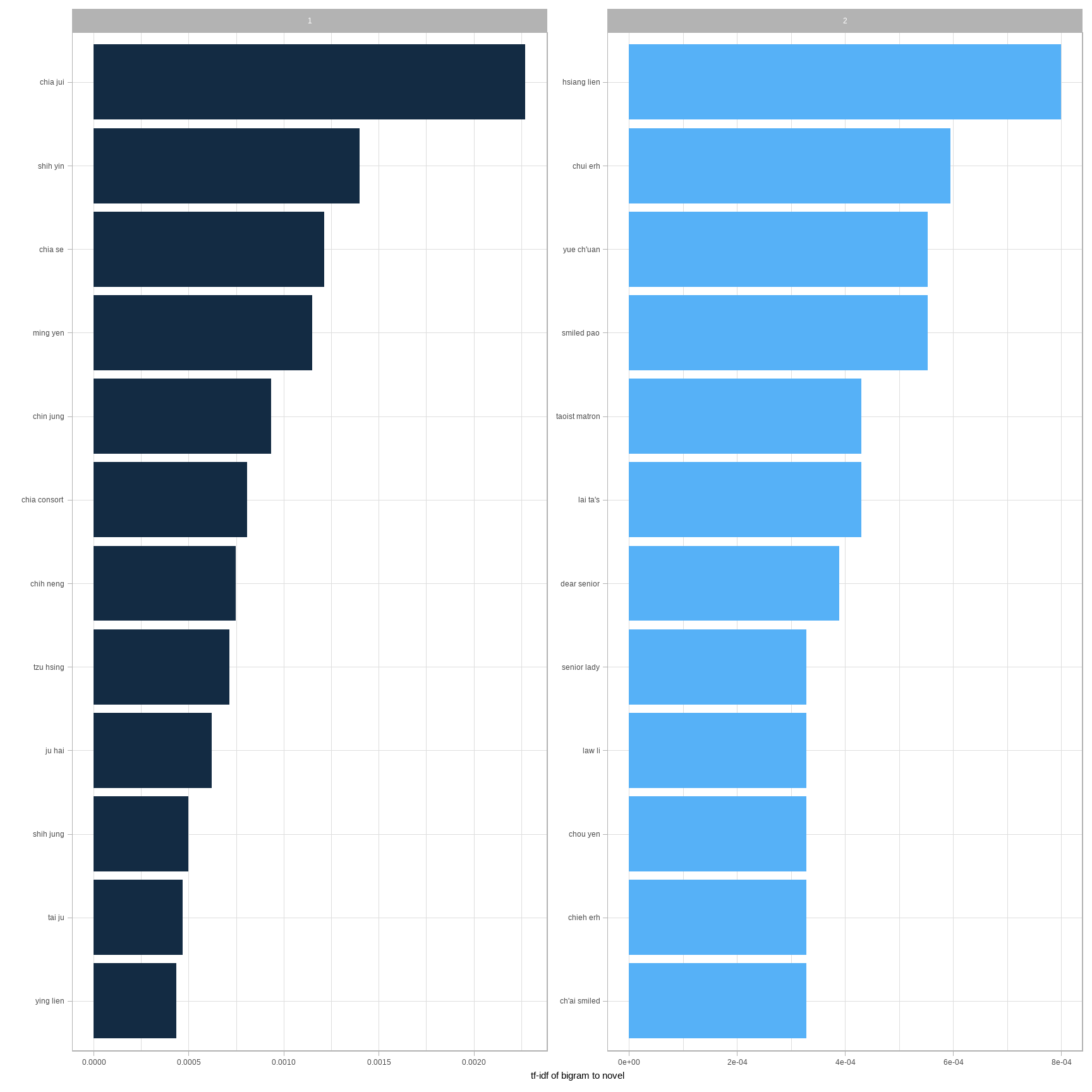
图 4.1: The 12 bigrams with the highest tf-idf from each half of Hongloumeng
Much as we discovered in Chapter 3, the units that distinguish each Austen book are almost exclusively names. We also notice some pairings of a common verb and a name, such as “replied elizabeth” in Pride & Prejudice, or “cried emma” in Emma.
There are advantages and disadvantages to examining the tf-idf of bigrams rather than individual words. Pairs of consecutive words might capture structure that isn’t present when one is just counting single words, and may provide context that makes tokens more understandable (for example, “pulteney street,” in Northanger Abbey, is more informative than “pulteney”). However, the per-bigram counts are also sparser: a typical two-word pair is rarer than either of its component words. Thus, bigrams can be especially useful when you have a very large text dataset.
4.1.3 使用二元组为情感分析提供上下文
Our sentiment analysis approach in Chapter 2 simply counted the appearance of positive or negative words, according to a reference lexicon. One of the problems with this approach is that a word’s context can matter nearly as much as its presence. For example, the words “happy” and “like” will be counted as positive, even in a sentence like “I’m not happy and I don’t like it!”
Now that we have the data organized into bigrams, it’s easy to tell how often words are preceded by a word like “not”:
bigrams_separated %>%
  filter(word1 == "not") %>%
  count(word1, word2, sort = TRUE)
## # A tibble: 540 x 3
## word1 word2 n
## <chr> <chr> <int>
## 1 not to 124
## 2 not be 97
## 3 not a 90
## 4 not have 53
## 5 not in 52
## 6 not even 38
## 7 not the 37
## 8 not as 35
## 9 not one 34
## 10 not only 33
## # ... with 530 more rowsBy performing sentiment analysis on the bigram data, we can examine how often sentiment-associated words are preceded by “not” or other negating words. We could use this to ignore or even reverse their contribution to the sentiment score.
Let’s use the AFINN lexicon for sentiment analysis, which you may recall gives a numeric sentiment value for each word, with positive or negative numbers indicating the direction of the sentiment.
AFINN <- get_sentiments("afinn")
AFINN
## # A tibble: 2,477 x 2
## word value
## <chr> <dbl>
## 1 abandon -2
## 2 abandoned -2
## 3 abandons -2
## 4 abducted -2
## 5 abduction -2
## 6 abductions -2
## 7 abhor -3
## 8 abhorred -3
## 9 abhorrent -3
## 10 abhors -3
## # ... with 2,467 more rowsWe can then examine the most frequent words that were preceded by “not” and were associated with a sentiment.
not_words <- bigrams_separated %>%
  filter(word1 == "not") %>%
  inner_join(AFINN, by = c(word2 = "word")) %>%
  count(word2, value, sort = TRUE)
not_words
## # A tibble: 75 x 3
## word2 value n
## <chr> <dbl> <int>
## 1 help 2 23
## 2 like 2 12
## 3 allow 1 10
## 4 easy 1 8
## 5 escape -1 8
## 6 agree 1 5
## 7 feeling 1 5
## 8 afraid -2 4
## 9 accept 1 3
## 10 good 3 3
## # ... with 65 more rowsFor example, the most common sentiment-associated word to follow “not” was “like,” which would normally have a (positive) score of 2.
It’s worth asking which words contributed the most in the “wrong” direction. To compute that, we can multiply their value by the number of times they appear (so that a word with a value of +3 occurring 10 times has as much impact as a word with a sentiment value of +1 occurring 30 times). We visualize the result with a bar plot (Figure 4.2).
library(ggplot2)
not_words %>%
  mutate(contribution = n * value) %>%
  arrange(desc(abs(contribution))) %>%
  head(20) %>%
  mutate(word2 = reorder(word2, contribution)) %>%
  ggplot(aes(word2, n * value, fill = n * value > 0)) +
  geom_col(show.legend = FALSE) +
  xlab("Words preceded by \"not\"") +
  ylab("Sentiment value * number of occurrences") +
  coord_flip()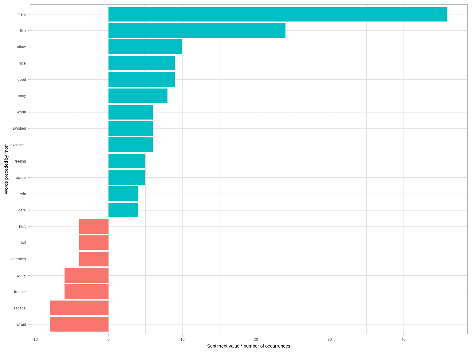
图 4.2: The 20 words preceded by ‘not’ that had the greatest contribution to sentiment values, in either a positive or negative direction
The bigrams “not like” and “not help” were overwhelmingly the largest causes of misidentification, making the text seem much more positive than it is. But we can see phrases like “not afraid” and “not fail” sometimes suggest text is more negative than it is.
“Not” isn’t the only term that provides some context for the following word. We could pick four common words (or more) that negate the subsequent term, and use the same joining and counting approach to examine all of them at once.
negation_words <- c("not", "no", "never", "without")
negated_words <- bigrams_separated %>%
  filter(word1 %in% negation_words) %>%
  inner_join(AFINN, by = c(word2 = "word")) %>%
  count(word1, word2, value, sort = TRUE)
We could then visualize what the most common words to follow each particular negation are (Figure 4.3). While “not like” and “not help” are still the two most common examples, we can also see pairings such as “no great” and “never loved.” We could combine this with the approaches in Chapter 2 to reverse the AFINN values of each word that follows a negation. These are just a few examples of how finding consecutive words can give context to text mining methods.
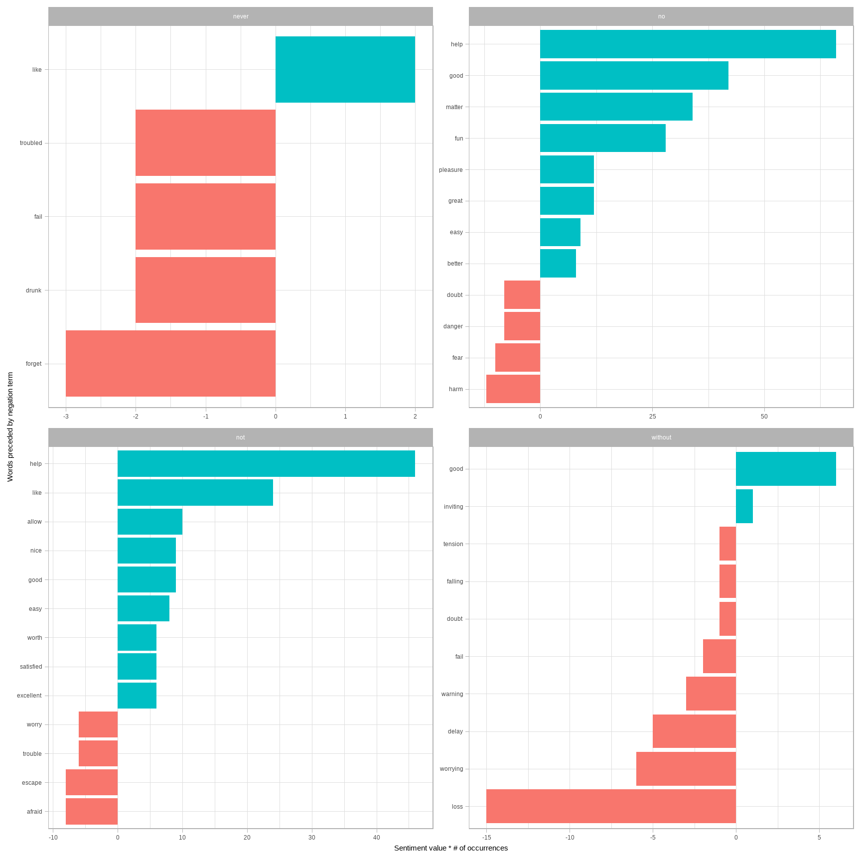
图 4.3: The most common positive or negative words to follow negations such as ‘never,’ ‘no,’ ‘not,’ and ‘without’
4.1.4 用 ggraph 绘制二元组网络
We may be interested in visualizing all of the relationships among words simultaneously, rather than just the top few at a time. As one common visualization, we can arrange the words into a network, or “graph.” Here we’ll be referring to a “graph” not in the sense of a visualization, but as a combination of connected nodes. A graph can be constructed from a tidy object since it has three variables:
- from: the node an edge is coming from
- to: the node an edge is going towards
- weight: A numeric value associated with each edge
The igraph package has many powerful functions for manipulating and analyzing networks. One way to create an igraph object from tidy data is the graph_from_data_frame() function, which takes a data frame of edges with columns for “from,” “to,” and edge attributes (in this case n):
library(igraph)

# original counts
bigram_counts
## # A tibble: 25,811 x 3
## word1 word2 n
## <chr> <chr> <int>
## 1 <NA> <NA> 8786
## 2 pao yue 1936
## 3 lady feng 820
## 4 tai yue 672
## 5 lady chia 616
## 6 pao ch'ai 555
## 7 hsi jen 482
## 8 dowager lady 448
## 9 madame wang 390
## 10 p'ing erh 297
## # ... with 25,801 more rows# filter for only relatively common combinations
bigram_graph <- bigram_counts %>%
filter(n > 25) %>%
graph_from_data_frame()
bigram_graph## IGRAPH b4e2387 DN-- 106 92 --
## + attr: name (v/c), n (e/n)
## + edges from b4e2387 (vertex names):
## [1] NA ->NA pao ->yue lady ->feng tai ->yue lady ->chia pao ->ch'ai
## [7] hsi ->jen dowager->lady madame ->wang p'ing ->erh hsiang ->yuen chia ->cheng
## [13] goody ->liu chia ->chen li ->wan lin ->tai t'an ->ch'un chia ->lien
## [19] hsueeh ->p'an yuean ->yang ch'ing ->wen yue ->ts'un waiting->maids chia ->jung
## [25] madame ->hsing pao ->yue's caught ->sight ch'in ->chung chia ->yuen waiting->maid
## [31] hsiang ->ling chia ->jui hsiao ->hung chou ->jui's servant->girls shih ->hsiang
## [37] cousin ->pao lady ->chia's jui's ->wife ying ->ch'un pei ->ming ying ->erh
## [43] ch'uan ->erh pao ->ch'in servant->girl madame ->wang's
## + ... omitted several edgesigraph has plotting functions built in, but they’re not what the package is designed to do, so many other packages have developed visualization methods for graph objects. We recommend the ggraph package (Pedersen 2021), because it implements these visualizations in terms of the grammar of graphics, which we are already familiar with from ggplot2.
We can convert an igraph object into a ggraph with the ggraph function, after which we add layers to it, much like layers are added in ggplot2. For example, for a basic graph we need to add three layers: nodes, edges, and text.
library(ggraph)
set.seed(2017)

ggraph(bigram_graph, layout = "fr") +
  geom_edge_link() +
  geom_node_point() +
  geom_node_text(aes(label = name), vjust = 1, hjust = 1)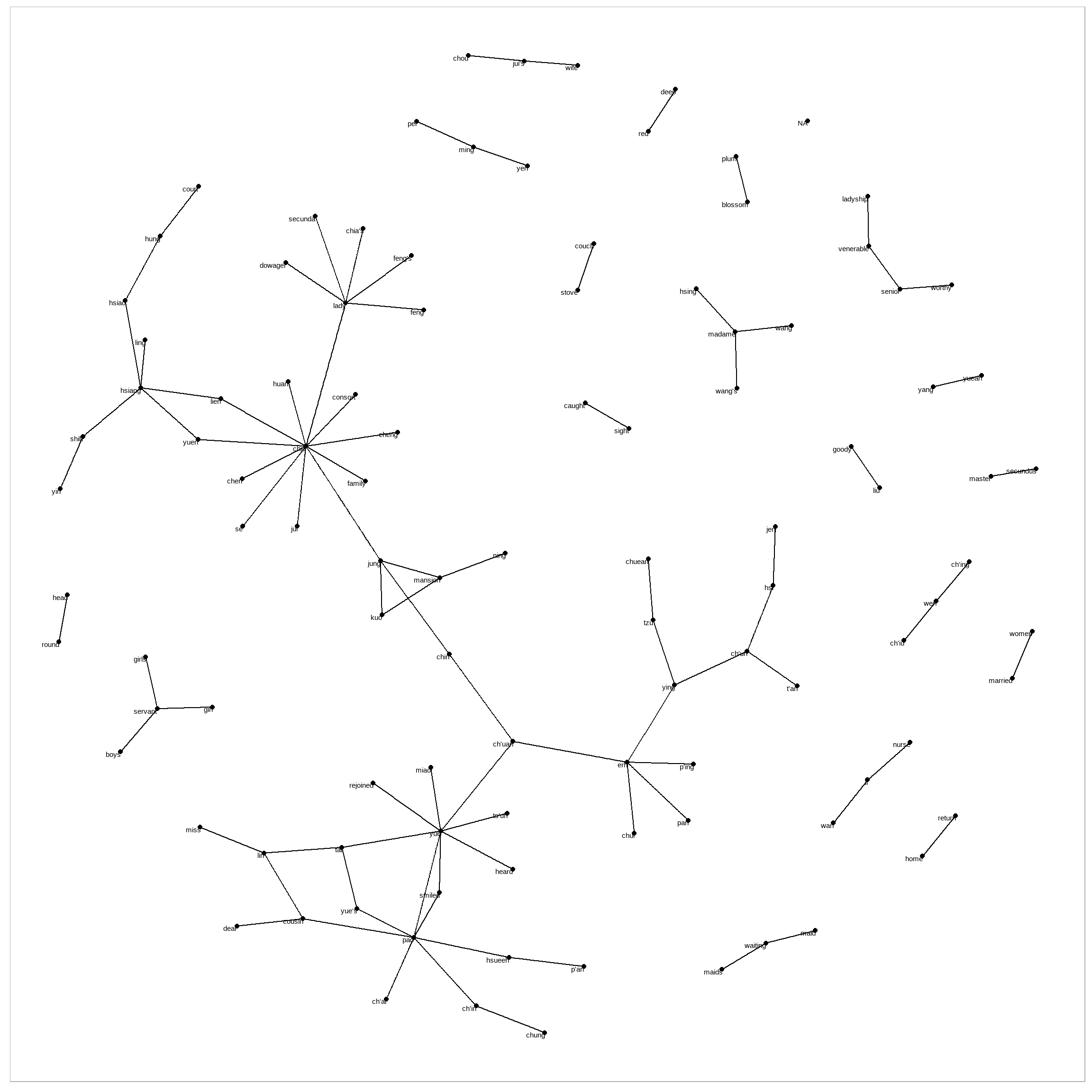
图 4.4: Common bigrams in Hongloumeng, showing those that occurred more than 25 times and where neither word was a stop word
In Figure 4.4, we can visualize some details of the text structure. For example, we see that salutations such as “miss,” “lady,” “sir,” “and”colonel" form common centers of nodes, which are often followed by names. We also see pairs or triplets along the outside that form common short phrases (“half hour,” “thousand pounds,” or “short time/pause”).
We conclude with a few polishing operations to make a better looking graph (Figure 4.5):
- We add the
edge_alphaaesthetic to the link layer to make links transparent based on how common or rare the bigram is - We add directionality with an arrow, constructed using
grid::arrow(), including anend_capoption that tells the arrow to end before touching the node - We tinker with the options to the node layer to make the nodes more attractive (larger, blue points)
- We add a theme that’s useful for plotting networks,
theme_void()
set.seed(2016)

a <- grid::arrow(type = "closed", length = unit(.15, "inches"))

ggraph(bigram_graph, layout = "fr") +
  geom_edge_link(aes(edge_alpha = n), show.legend = FALSE,
                 arrow = a, end_cap = circle(.07, 'inches')) +
  geom_node_point(color = "lightblue", size = 5) +
  geom_node_text(aes(label = name), vjust = 1, hjust = 1) +
  theme_void()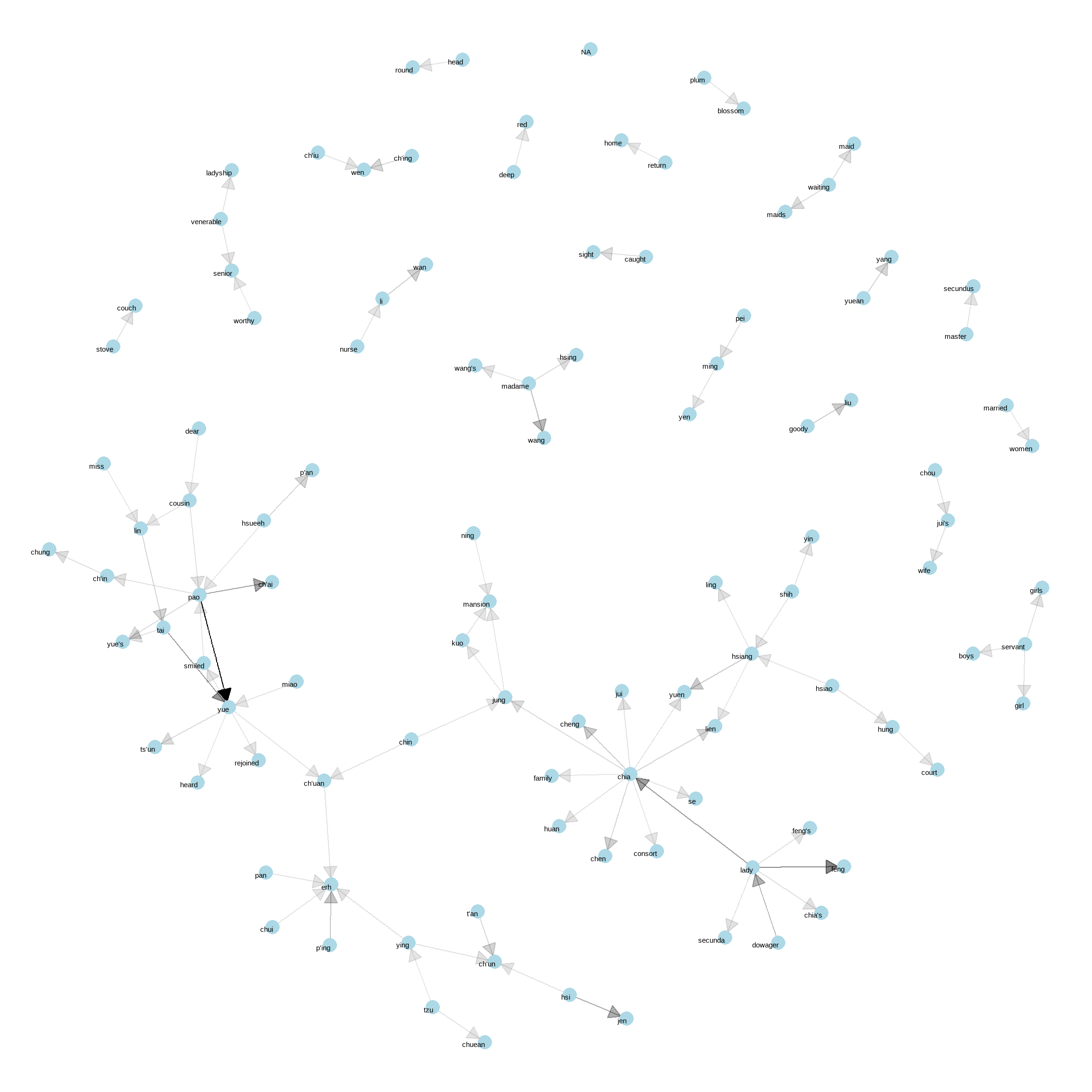
图 4.5: Common bigrams in Hongloumeng, with some polishing
It may take some experimentation with ggraph to get your networks into a presentable format like this, but the network structure is useful and flexible way to visualize relational tidy data.
Note that this is a visualization of a Markov chain, a common model in text processing. In a Markov chain, each choice of word depends only on the previous word. In this case, a random generator following this model might spit out “dear,” then “sir,” then “william/walter/thomas/thomas’s,” by following each word to the most common words that follow it. To make the visualization interpretable, we chose to show only the most common word to word connections, but one could imagine an enormous graph representing all connections that occur in the text.
4.1.5 绘制其它文本的二元组
We went to a good amount of work in cleaning and visualizing bigrams on a text dataset, so let’s collect it into a function so that we easily perform it on other text datasets.
To make it easy to use the count_bigrams() and visualize_bigrams() yourself, we’ve also reloaded the packages necessary for them.
library(dplyr)
library(tidyr)
library(tidytext)
library(ggplot2)
library(igraph)
library(ggraph)

count_bigrams <- function(dataset) {
  dataset %>%
    unnest_tokens(bigram, text, token = "ngrams", n = 2) %>%
    separate(bigram, c("word1", "word2"), sep = " ") %>%
    filter(!word1 %in% stop_words$word,
           !word2 %in% stop_words$word) %>%
    count(word1, word2, sort = TRUE)
}

visualize_bigrams <- function(bigrams) {
  set.seed(2016)
  a <- grid::arrow(type = "closed", length = unit(.15, "inches"))

  bigrams %>%
    graph_from_data_frame() %>%
    ggraph(layout = "fr") +
    geom_edge_link(aes(edge_alpha = n), show.legend = FALSE, arrow = a) +
    geom_node_point(color = "lightblue", size = 5) +
    geom_node_text(aes(label = name), vjust = 1, hjust = 1) +
    theme_void()
}
At this point, we could visualize bigrams in other works, such as the King James Version of the Bible:
# the King James version is book 10 on Project Gutenberg:
library(gutenbergr)
kjv <- gutenberg_download(10)library(stringr)
kjv_bigrams <- kjv %>%
count_bigrams()
# filter out rare combinations, as well as digits
kjv_bigrams %>%
filter(n > 40,
!str_detect(word1, "\\d"),
!str_detect(word2, "\\d")) %>%
visualize_bigrams()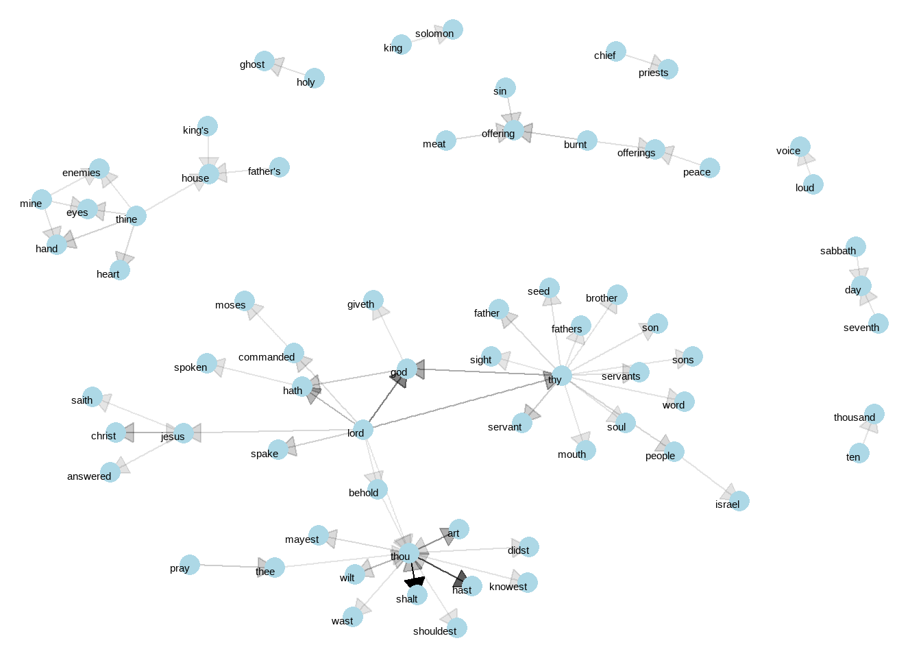
图 4.6: Directed graph of common bigrams in the King James Bible, showing those that occurred more than 40 times
Figure 4.6 thus lays out a common “blueprint” of language within the Bible, particularly focused around “thy” and “thou” (which could probably be considered stopwords!) You can use the gutenbergr package and these count_bigrams/visualize_bigrams functions to visualize bigrams in other classic books you’re interested in.
4.2 用 widyr 包计算和关联词对
Tokenizing by n-gram is a useful way to explore pairs of adjacent words. However, we may also be interested in words that tend to co-occur within particular documents or particular chapters, even if they don’t occur next to each other.
Tidy data is a useful structure for comparing between variables or grouping by rows, but it can be challenging to compare between rows: for example, to count the number of times that two words appear within the same document, or to see how correlated they are. Most operations for finding pairwise counts or correlations need to turn the data into a wide matrix first.
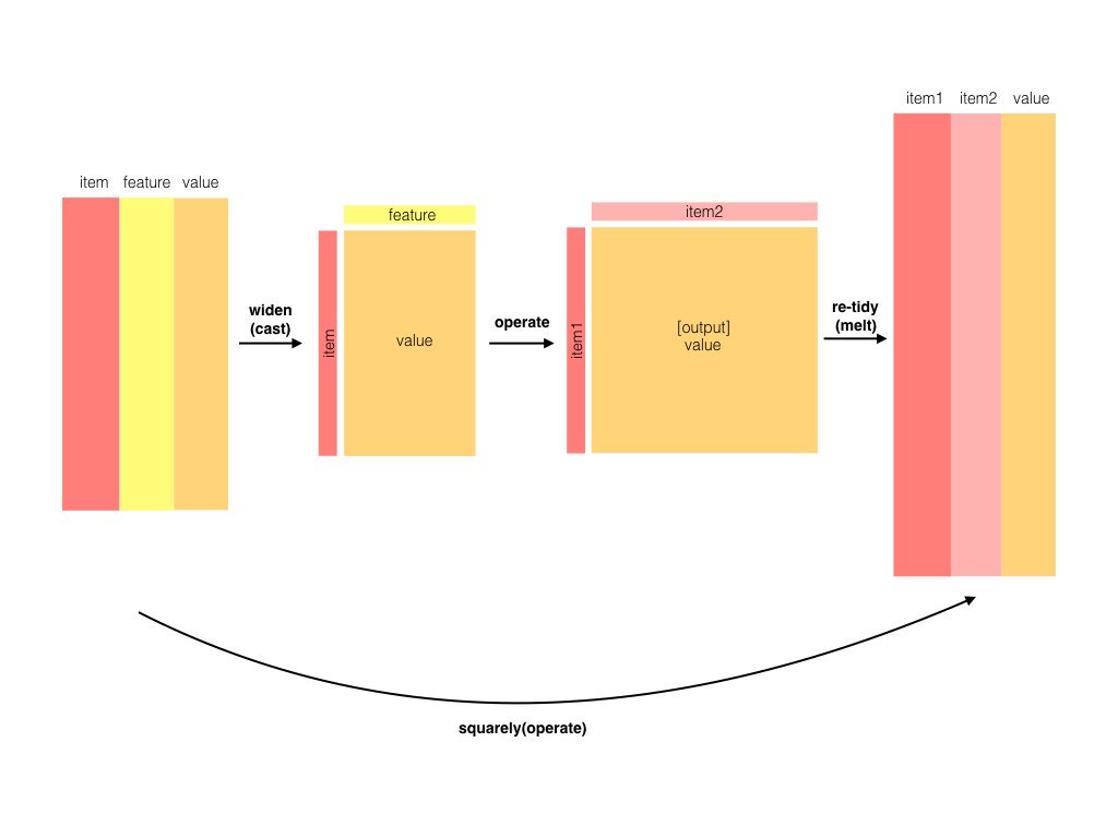
图 4.7: The philosophy behind the widyr package, which can perform operations such as counting and correlating on pairs of values in a tidy dataset. The widyr package first ‘casts’ a tidy dataset into a wide matrix, performs an operation such as a correlation on it, then re-tidies the result.
We’ll examine some of the ways tidy text can be turned into a wide matrix in Chapter 5, but in this case it isn’t necessary. The widyr package makes operations such as computing counts and correlations easy, by simplifying the pattern of “widen data, perform an operation, then re-tidy data” (Figure 4.7). We’ll focus on a set of functions that make pairwise comparisons between groups of observations (for example, between documents, or sections of text).
4.2.1 在段落间计算和关联
Consider the book “Pride and Prejudice” divided into 10-line sections, as we did (with larger sections) for sentiment analysis in Chapter 2. We may be interested in what words tend to appear within the same section.
library(stringi)

section_words <- hongloumeng_en %>%
  mutate(book = cumsum(str_detect(text, regex("HUNG LOU MENG, BOOK [I]+")))) %>%
  mutate(section = row_number() %/% 10) %>%
  filter(section > 0) %>%
  unnest_tokens(word, text) %>%
  filter(!word %in% stop_words$word)
section_words
## # A tibble: 160,233 x 5
## gutenberg_id title book section word
## <int> <chr> <int> <dbl> <chr>
## 1 9603 Hung Lou Meng, or, the Dream of the Red Chamber, a Chinese~ 1 1 book
## 2 9603 Hung Lou Meng, or, the Dream of the Red Chamber, a Chinese~ 1 2 preface
## 3 9603 Hung Lou Meng, or, the Dream of the Red Chamber, a Chinese~ 1 2 translati~
## 4 9603 Hung Lou Meng, or, the Dream of the Red Chamber, a Chinese~ 1 2 suggested
## 5 9603 Hung Lou Meng, or, the Dream of the Red Chamber, a Chinese~ 1 2 pretensio~
## 6 9603 Hung Lou Meng, or, the Dream of the Red Chamber, a Chinese~ 1 2 range
## 7 9603 Hung Lou Meng, or, the Dream of the Red Chamber, a Chinese~ 1 2 ranks
## 8 9603 Hung Lou Meng, or, the Dream of the Red Chamber, a Chinese~ 1 2 body
## 9 9603 Hung Lou Meng, or, the Dream of the Red Chamber, a Chinese~ 1 2 sinologues
## 10 9603 Hung Lou Meng, or, the Dream of the Red Chamber, a Chinese~ 1 2 perplexit~
## # ... with 160,223 more rowsOne useful function from widyr is the pairwise_count() function. The prefix pairwise_ means it will result in one row for each pair of words in the word variable. This lets us count common pairs of words co-appearing within the same section:
library(widyr)

# count words co-occuring within sections
word_pairs <- section_words %>%
  pairwise_count(word, section, sort = TRUE)
word_pairs
## # A tibble: 3,077,492 x 3
## item1 item2 n
## <chr> <chr> <dbl>
## 1 pao yue 1499
## 2 yue pao 1499
## 3 lady chia 732
## 4 chia lady 732
## 5 lady feng 698
## 6 feng lady 698
## 7 tai yue 544
## 8 yue tai 544
## 9 ch'ai pao 453
## 10 pao ch'ai 453
## # ... with 3,077,482 more rowsNotice that while the input had one row for each pair of a document (a 10-line section) and a word, the output has one row for each pair of words. This is also a tidy format, but of a very different structure that we can use to answer new questions.
For example, we can see that the most common pair of words in a section is “Elizabeth” and “Darcy” (the two main characters). We can easily find the words that most often occur with Darcy:
word_pairs %>%
  filter(item1 == "pao")
## # A tibble: 8,143 x 3
## item1 item2 n
## <chr> <chr> <dbl>
## 1 pao yue 1499
## 2 pao ch'ai 453
## 3 pao tai 392
## 4 pao chia 383
## 5 pao lady 381
## 6 pao time 333
## 7 pao hsi 297
## 8 pao day 292
## 9 pao jen 258
## 10 pao words 240
## # ... with 8,133 more rows4.2.2 词对的相关度
Pairs like “Elizabeth” and “Darcy” are the most common co-occurring words, but that’s not particularly meaningful since they’re also the most common individual words. We may instead want to examine correlation among words, which indicates how often they appear together relative to how often they appear separately.
In particular, here we’ll focus on the phi coefficient, a common measure for binary correlation. The focus of the phi coefficient is how much more likely it is that either both word X and Y appear, or neither do, than that one appears without the other.
Consider the following table:
| Has word Y | No word Y | Total | ||
|---|---|---|---|---|
| Has word X | \(n_{11}\) | \(n_{10}\) | \(n_{1\cdot}\) | |
| No word X | \(n_{01}\) | \(n_{00}\) | \(n_{0\cdot}\) | |
| Total | \(n_{\cdot 1}\) | \(n_{\cdot 0}\) | n |
For example, that \(n_{11}\) represents the number of documents where both word X and word Y appear, \(n_{00}\) the number where neither appears, and \(n_{10}\) and \(n_{01}\) the cases where one appears without the other. In terms of this table, the phi coefficient is:
\[\phi=\frac{n_{11}n_{00}-n_{10}n_{01}}{\sqrt{n_{1\cdot}n_{0\cdot}n_{\cdot0}n_{\cdot1}}}\]
The phi coefficient is equivalent to the Pearson correlation, which you may have heard of elsewhere, when it is applied to binary data).
The pairwise_cor() function in widyr lets us find the phi coefficient between words based on how often they appear in the same section. Its syntax is similar to pairwise_count().
# we need to filter for at least relatively common words first
word_cors <- section_words %>%
  group_by(word) %>%
  filter(n() >= 20) %>%
  pairwise_cor(word, section, sort = TRUE)
word_cors
## # A tibble: 2,613,072 x 3
## item1 item2 correlation
## <chr> <chr> <dbl>
## 1 goody liu 0.917
## 2 liu goody 0.917
## 3 hsi jen 0.868
## 4 jen hsi 0.868
## 5 vista broad 0.810
## 6 broad vista 0.810
## 7 t'an ch'un 0.788
## 8 ch'un t'an 0.788
## 9 yuean yang 0.772
## 10 yang yuean 0.772
## # ... with 2,613,062 more rowsThis output format is helpful for exploration. For example, we could find the words most correlated with a word like “pounds” using a filter operation.
word_cors %>%
  filter(item1 == "ounces")
## # A tibble: 1,616 x 3
## item1 item2 correlation
## <chr> <chr> <dbl>
## 1 ounces silver 0.201
## 2 ounces twenty 0.156
## 3 ounces hundred 0.125
## 4 ounces chiao 0.122
## 5 ounces thousand 0.116
## 6 ounces responded 0.103
## 7 ounces credit 0.103
## 8 ounces prepare 0.0961
## 9 ounces ten 0.0900
## 10 ounces powder 0.0887
## # ... with 1,606 more rowsThis lets us pick particular interesting words and find the other words most associated with them (Figure 4.8).
word_cors %>%
  filter(item1 %in% c("yue", "ounces", "married", "red")) %>%
  group_by(item1) %>%
  top_n(8) %>%
  ungroup() %>%
  mutate(item2 = reorder(item2, correlation)) %>%
  ggplot(aes(item2, correlation)) +
  geom_bar(stat = "identity") +
  facet_wrap(~ item1, scales = "free") +
  coord_flip()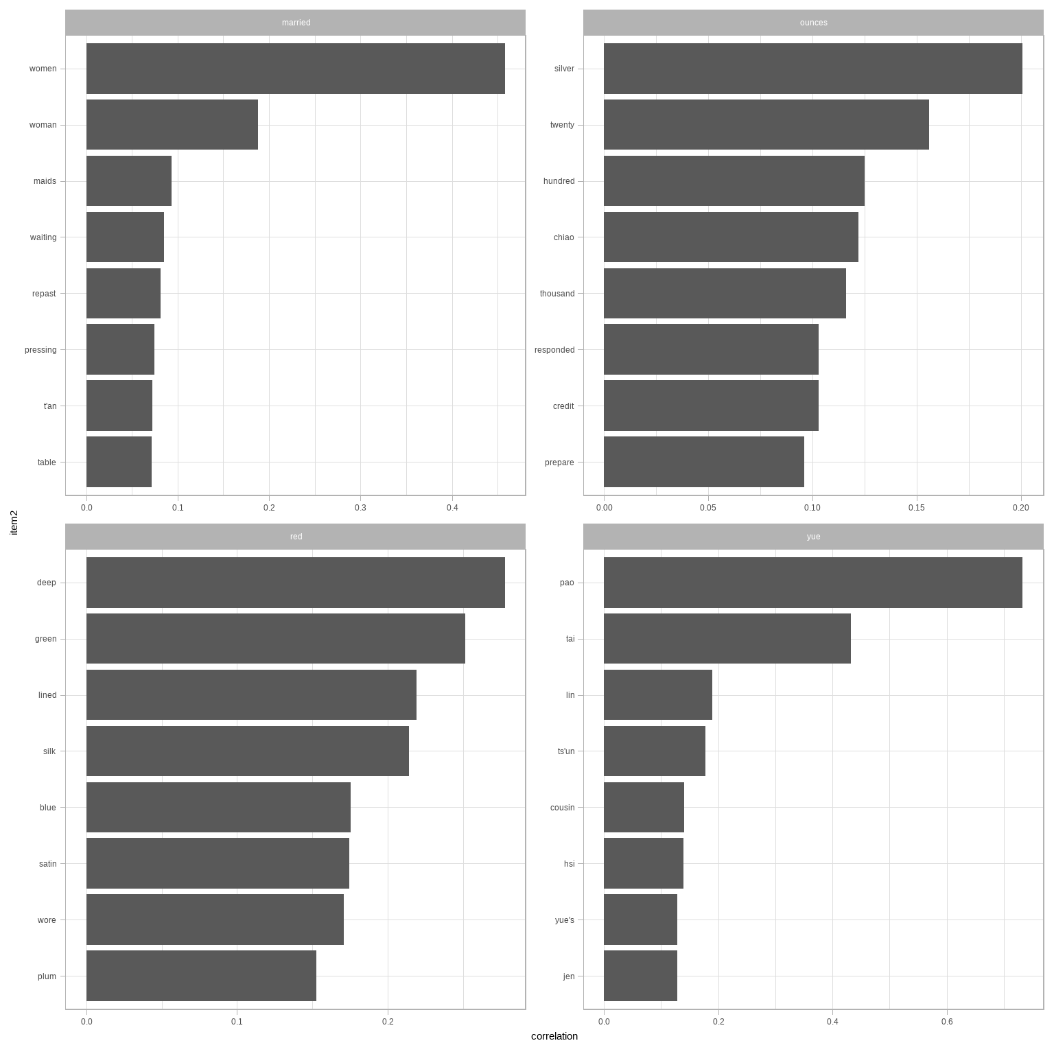
图 4.8: Words from Pride and Prejudice that were most correlated with ‘elizabeth,’ ‘pounds,’ ‘married,’ and ‘pride’
Just as we used ggraph to visualize bigrams, we can use it to visualize the correlations and clusters of words that were found by the widyr package (Figure 4.9).
set.seed(2016)

word_cors %>%
  filter(correlation > .20) %>%
  graph_from_data_frame() %>%
  ggraph(layout = "fr") +
  geom_edge_link(aes(edge_alpha = correlation), show.legend = FALSE) +
  geom_node_point(color = "lightblue", size = 5) +
  geom_node_text(aes(label = name), repel = TRUE) +
  theme_void()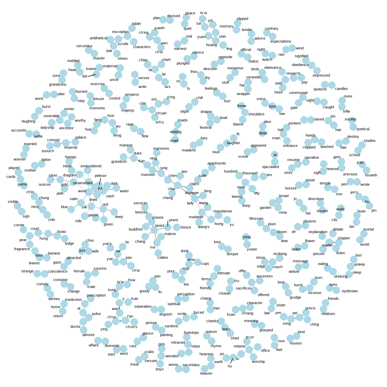
图 4.9: Pairs of words in Pride and Prejudice that show at least a .15 correlation of appearing within the same 10-line section
Note that unlike the bigram analysis, the relationships here are symmetrical, rather than directional (there are no arrows). We can also see that while pairings of names and titles that dominated bigram pairings are common, such as “colonel/fitzwilliam,” we can also see pairings of words that appear close to each other, such as “walk” and “park,” or “dance” and “ball.”
4.3 小结
This chapter showed how the tidy text approach is useful not only for analyzing individual words, but also for exploring the relationships and connections between words. Such relationships can involve n-grams, which enable us to see what words tend to appear after others, or co-occurences and correlations, for words that appear in proximity to each other. This chapter also demonstrated the ggraph package for visualizing both of these types of relationships as networks. These network visualizations are a flexible tool for exploring relationships, and will play an important role in the case studies in later chapters.