第 5 章 非 tidy 格式与 tidy 格式互相转换
In the previous chapters, we’ve been analyzing text arranged in the tidy text format: a table with one-token-per-document-per-row, such as is constructed by the unnest_tokens() function. This lets us use the popular suite of tidy tools such as dplyr, tidyr, and ggplot2 to explore and visualize text data. We’ve demonstrated that many informative text analyses can be performed using these tools.
However, most of the existing R tools for natural language processing, besides the tidytext package, aren’t compatible with this format. The CRAN Task View for Natural Language Processing lists a large selection of packages that take other structures of input and provide non-tidy outputs. These packages are very useful in text mining applications, and many existing text datasets are structured according to these formats.
Computer scientist Hal Abelson has observed that “No matter how complex and polished the individual operations are, it is often the quality of the glue that most directly determines the power of the system” (Abelson 2008). In that spirit, this chapter will discuss the “glue” that connects the tidy text format with other important packages and data structures, allowing you to rely on both existing text mining packages and the suite of tidy tools to perform your analysis.
图 5.1: A flowchart of a typical text analysis that combines tidytext with other tools and data formats, particularly the tm or quanteda packages. This chapter shows how to convert back and forth between document-term matrices and tidy data frames, as well as converting from a Corpus object to a text data frame.
Figure 5.1 illustrates how an analysis might switch between tidy and non-tidy data structures and tools. This chapter will focus on the process of tidying document-term matrices, as well as casting a tidy data frame into a sparse matrix. We’ll also explore how to tidy Corpus objects, which combine raw text with document metadata, into text data frames, leading to a case study of ingesting and analyzing financial articles.
5.1 将文档-术语矩阵 tidy 化
One of the most common structures that text mining packages work with is the document-term matrix (or DTM). This is a matrix where:
- each row represents one document (such as a book or article),
- each column represents one term, and
- each value (typically) contains the number of appearances of that term in that document.
Since most pairings of document and term do not occur (they have the value zero), DTMs are usually implemented as sparse matrices. These objects can be treated as though they were matrices (for example, accessing particular rows and columns), but are stored in a more efficient format. We’ll discuss several implementations of these matrices in this chapter.
DTM objects cannot be used directly with tidy tools, just as tidy data frames cannot be used as input for most text mining packages. Thus, the tidytext package provides two verbs that convert between the two formats.
tidy()turns a document-term matrix into a tidy data frame. This verb comes from the broom package (Robinson, Hayes, and Couch 2021), which provides similar tidying functions for many statistical models and objects.cast()turns a tidy one-term-per-row data frame into a matrix. tidytext provides three variations of this verb, each converting to a different type of matrix:cast_sparse()(converting to a sparse matrix from the Matrix package),cast_dtm()(converting to aDocumentTermMatrixobject from tm), andcast_dfm()(converting to adfmobject from quanteda).
As shown in Figure 5.1, a DTM is typically comparable to a tidy data frame after a count or a group_by/summarize that contains counts or another statistic for each combination of a term and document.
5.1.1 将 DocumentTermMatrix 对象 tidy 化
Perhaps the most widely used implementation of DTMs in R is the DocumentTermMatrix class in the tm package. Many available text mining datasets are provided in this format. For example, consider the collection of Associated Press newspaper articles included in the topicmodels package.
library(tm)

data("AssociatedPress", package = "topicmodels")
AssociatedPress
## <<DocumentTermMatrix (documents: 2246, terms: 10473)>>
## Non-/sparse entries: 302031/23220327
## Sparsity : 99%
## Maximal term length: 18
## Weighting : term frequency (tf)We see that this dataset contains 2246 documents (each of them an AP article) and 10473 terms (distinct words). Notice that this DTM is 99% sparse (99% of document-word pairs are zero). We could access the terms in the document with the Terms() function.
terms <- Terms(AssociatedPress)
head(terms)
## [1] "aaron" "abandon" "abandoned" "abandoning" "abbott" "abboud"If we wanted to analyze this data with tidy tools, we would first need to turn it into a data frame with one-token-per-document-per-row. The broom package introduced the tidy() verb, which takes a non-tidy object and turns it into a tidy data frame. The tidytext package implements this method for DocumentTermMatrix objects.
library(dplyr)
library(tidytext)

ap_td <- tidy(AssociatedPress)
ap_td
## # A tibble: 302,031 x 3
## document term count
## <int> <chr> <dbl>
## 1 1 adding 1
## 2 1 adult 2
## 3 1 ago 1
## 4 1 alcohol 1
## 5 1 allegedly 1
## 6 1 allen 1
## 7 1 apparently 2
## 8 1 appeared 1
## 9 1 arrested 1
## 10 1 assault 1
## # ... with 302,021 more rowsNotice that we now have a tidy three-column tbl_df, with variables document, term, and count. This tidying operation is similar to the melt() function from the reshape2 package (Wickham 2020) for non-sparse matrices.
Notice that only the non-zero values are included in the tidied output: document 1 includes terms such as “adding” and “adult,” but not “aaron” or “abandon.” This means the tidied version has no rows where count is zero.
As we’ve seen in previous chapters, this form is convenient for analysis with the dplyr, tidytext and ggplot2 packages. For example, you can perform sentiment analysis on these newspaper articles with the approach described in Chapter 2.
ap_sentiments <- ap_td %>%
  inner_join(get_sentiments("bing"), by = c(term = "word"))

ap_sentiments
## # A tibble: 30,094 x 4
## document term count sentiment
## <int> <chr> <dbl> <chr>
## 1 1 assault 1 negative
## 2 1 complex 1 negative
## 3 1 death 1 negative
## 4 1 died 1 negative
## 5 1 good 2 positive
## 6 1 illness 1 negative
## 7 1 killed 2 negative
## 8 1 like 2 positive
## 9 1 liked 1 positive
## 10 1 miracle 1 positive
## # ... with 30,084 more rowsThis would let us visualize which words from the AP articles most often contributed to positive or negative sentiment, seen in Figure 5.2. We can see that the most common positive words include “like,” “work,” “support,” and “good,” while the most negative words include “killed,” “death,” and “vice.” (The inclusion of “vice” as a negative term is probably a mistake on the algorithm’s part, since it likely usually refers to “vice president”).
library(ggplot2)

ap_sentiments %>%
  count(sentiment, term, wt = count) %>%
  ungroup() %>%
  filter(n >= 200) %>%
  mutate(n = ifelse(sentiment == "negative", -n, n)) %>%
  mutate(term = reorder(term, n)) %>%
  ggplot(aes(term, n, fill = sentiment)) +
  geom_bar(stat = "identity") +
  ylab("Contribution to sentiment") +
  coord_flip()
图 5.2: Words from AP articles with the greatest contribution to positive or negative sentiments, using the Bing sentiment lexicon.
5.1.2 将 dfm 对象 tidy 化
Other text mining packages provide alternative implementations of document-term matrices, such as the dfm (document-feature matrix) class from the quanteda package (Benoit et al. 2020). For example, the quanteda package comes with a corpus of presidential inauguration speeches, which can be converted to a dfm using the appropriate function.
data("data_corpus_inaugural", package = "quanteda")
inaug_dfm <- quanteda::dfm(data_corpus_inaugural, verbose = FALSE)inaug_dfm## Document-feature matrix of: 58 documents, 9,360 features (91.8% sparse) and 4 docvars.
## features
## docs fellow-citizens of the senate and house representatives : among vicissitudes
## 1789-Washington 1 71 116 1 48 2 2 1 1 1
## 1793-Washington 0 11 13 0 2 0 0 1 0 0
## 1797-Adams 3 140 163 1 130 0 2 0 4 0
## 1801-Jefferson 2 104 130 0 81 0 0 1 1 0
## 1805-Jefferson 0 101 143 0 93 0 0 0 7 0
## 1809-Madison 1 69 104 0 43 0 0 0 0 0
## [ reached max_ndoc ... 52 more documents, reached max_nfeat ... 9,350 more features ]The tidy method works on these document-feature matrices as well, turning them into a one-token-per-document-per-row table:
inaug_td <- tidy(inaug_dfm)
inaug_td
## # A tibble: 44,710 x 3
## document term count
## <chr> <chr> <dbl>
## 1 1789-Washington fellow-citizens 1
## 2 1797-Adams fellow-citizens 3
## 3 1801-Jefferson fellow-citizens 2
## 4 1809-Madison fellow-citizens 1
## 5 1813-Madison fellow-citizens 1
## 6 1817-Monroe fellow-citizens 5
## 7 1821-Monroe fellow-citizens 1
## 8 1841-Harrison fellow-citizens 11
## 9 1845-Polk fellow-citizens 1
## 10 1849-Taylor fellow-citizens 1
## # ... with 44,700 more rowsWe may be interested in finding the words most specific to each of the inaugural speeches. This could be quantified by calculating the tf-idf of each term-speech pair using the bind_tf_idf() function, as described in Chapter 3.
inaug_tf_idf <- inaug_td %>%
  bind_tf_idf(term, document, count) %>%
  arrange(desc(tf_idf))

inaug_tf_idf
## # A tibble: 44,710 x 6
## document term count tf idf tf_idf
## <chr> <chr> <dbl> <dbl> <dbl> <dbl>
## 1 1793-Washington arrive 1 0.00680 4.06 0.0276
## 2 1793-Washington upbraidings 1 0.00680 4.06 0.0276
## 3 1793-Washington violated 1 0.00680 3.37 0.0229
## 4 1793-Washington willingly 1 0.00680 3.37 0.0229
## 5 1793-Washington incurring 1 0.00680 3.37 0.0229
## 6 1793-Washington previous 1 0.00680 2.96 0.0201
## 7 1793-Washington knowingly 1 0.00680 2.96 0.0201
## 8 1793-Washington injunctions 1 0.00680 2.96 0.0201
## 9 1793-Washington witnesses 1 0.00680 2.96 0.0201
## 10 1793-Washington besides 1 0.00680 2.67 0.0182
## # ... with 44,700 more rowsWe could use this data to pick four notable inaugural addresses (from Presidents Lincoln, Roosevelt, Kennedy, and Obama), and visualize the words most specific to each speech, as shown in Figure 5.3.
图 5.3: The terms with the highest tf-idf from each of four selected inaugural addresses. Note that quanteda’s tokenizer includes the ‘?’ punctuation mark as a term, though the texts we’ve tokenized ourselves with unnest_tokens do not.
As another example of a visualization possible with tidy data, we could extract the year from each document’s name, and compute the total number of words within each year.
Note that we’ve used tidyr’s complete() function to include zeroes (cases where a word didn’t appear in a document) in the table.
library(tidyr)

year_term_counts <- inaug_td %>%
  extract(document, "year", "(\\d+)", convert = TRUE) %>%
  complete(year, term, fill = list(count = 0)) %>%
  group_by(year) %>%
  mutate(year_total = sum(count))
This lets us pick several words and visualize how they changed in frequency over time, as shown in 5.4. We can see that over time, American presidents became less likely to refer to the country as the “Union” and more likely to refer to “America.” They also became less likely to talk about the “constitution” and foreign" countries, and more likely to mention “freedom” and “God.”
year_term_counts %>%
  filter(term %in% c("god", "america", "foreign", "union", "constitution", "freedom")) %>%
  ggplot(aes(year, count / year_total)) +
  geom_point() +
  geom_smooth() +
  facet_wrap(~ term, scales = "free_y") +
  scale_y_continuous(labels = scales::percent_format()) +
  ylab("% frequency of word in inaugural address")
图 5.4: Changes in word frequency over time within Presidential inaugural addresses, for six selected terms
These examples show how you can use tidytext, and the related suite of tidy tools, to analyze sources even if their origin was not in a tidy format.
5.2 将 tidy 文本数据投射至矩阵
Just as some existing text mining packages provide document-term matrices as sample data or output, some algorithms expect such matrices as input. Therefore, tidytext provides cast_ verbs for converting from a tidy form to these matrices.
For example, we could take the tidied AP dataset and cast it back into a document-term matrix using the cast_dtm() function.
ap_td %>%
  cast_dtm(document, term, count)
## <<DocumentTermMatrix (documents: 2246, terms: 10473)>>
## Non-/sparse entries: 302031/23220327
## Sparsity : 99%
## Maximal term length: 18
## Weighting : term frequency (tf)Similarly, we could cast the table into a dfm object from quanteda’s dfm with cast_dfm().
ap_td %>%
  cast_dfm(document, term, count)
## Document-feature matrix of: 2,246 documents, 10,473 features (98.7% sparse).
## features
## docs adding adult ago alcohol allegedly allen apparently appeared arrested assault
## 1 1 2 1 1 1 1 2 1 1 1
## 2 0 0 0 0 0 0 0 1 0 0
## 3 0 0 1 0 0 0 0 1 0 0
## 4 0 0 3 0 0 0 0 0 0 0
## 5 0 0 0 0 0 0 0 0 0 0
## 6 0 0 2 0 0 0 0 0 0 0
## [ reached max_ndoc ... 2,240 more documents, reached max_nfeat ... 10,463 more features ]Some tools simply require a sparse matrix:
library(Matrix)

# cast into a Matrix object
m <- ap_td %>%
  cast_sparse(document, term, count)

class(m)
## [1] "dgCMatrix"
## attr(,"package")
## [1] "Matrix"dim(m)## [1] 2246 10473This kind of conversion could easily be done from any of the tidy text structures we’ve used so far in this book. For example, we could create a DTM of Jane Austen’s books in just a few lines of code.
library(janeaustenr)

austen_dtm <- austen_books() %>%
  unnest_tokens(word, text) %>%
  count(book, word) %>%
  cast_dtm(book, word, n)

austen_dtm
## <<DocumentTermMatrix (documents: 6, terms: 14520)>>
## Non-/sparse entries: 40379/46741
## Sparsity : 54%
## Maximal term length: 19
## Weighting : term frequency (tf)This casting process allows for reading, filtering, and processing to be done using dplyr and other tidy tools, after which the data can be converted into a document-term matrix for machine learning applications. In Chapter 6, we’ll examine some examples where a tidy-text dataset has to be converted into a DocumentTermMatrix for processing.
5.3 将带有元数据的语料对象 tidy 化
Some data structures are designed to store document collections before tokenization, often called a “corpus.” One common example is Corpus objects from the tm package. These store text alongside metadata, which may include an ID, date/time, title, or language for each document.
For example, the tm package comes with the acq corpus, containing 50 articles from the news service Reuters.
data("acq")
acq
## <<VCorpus>>
## Metadata: corpus specific: 0, document level (indexed): 0
## Content: documents: 50# first document
acq[[1]]## <<PlainTextDocument>>
## Metadata: 15
## Content: chars: 1287A corpus object is structured like a list, with each item containing both text and metadata (see the tm documentation for more on working with Corpus documents). This is a flexible storage method for documents, but doesn’t lend itself to processing with tidy tools.
We can thus use the tidy() method to construct a table with one row per document, including the metadata (such as id and datetimestamp) as columns alongside the text.
acq_td <- tidy(acq)
acq_td
## # A tibble: 50 x 16
## author datetimestamp description heading id language origin topics lewissplit cgisplit
## <chr> <dttm> <chr> <chr> <chr> <chr> <chr> <chr> <chr> <chr>
## 1 <NA> 1987-02-26 23:18:06 "" COMPUTE~ 10 en Reute~ YES TRAIN TRAININ~
## 2 <NA> 1987-02-26 23:19:15 "" OHIO MA~ 12 en Reute~ YES TRAIN TRAININ~
## 3 <NA> 1987-02-26 23:49:56 "" MCLEAN'~ 44 en Reute~ YES TRAIN TRAININ~
## 4 By Cal~ 1987-02-26 23:51:17 "" CHEMLAW~ 45 en Reute~ YES TRAIN TRAININ~
## 5 <NA> 1987-02-27 00:08:33 "" <COFAB ~ 68 en Reute~ YES TRAIN TRAININ~
## 6 <NA> 1987-02-27 00:32:37 "" INVESTM~ 96 en Reute~ YES TRAIN TRAININ~
## 7 By Pat~ 1987-02-27 00:43:13 "" AMERICA~ 110 en Reute~ YES TRAIN TRAININ~
## 8 <NA> 1987-02-27 00:59:25 "" HONG KO~ 125 en Reute~ YES TRAIN TRAININ~
## 9 <NA> 1987-02-27 01:01:28 "" LIEBERT~ 128 en Reute~ YES TRAIN TRAININ~
## 10 <NA> 1987-02-27 01:08:27 "" GULF AP~ 134 en Reute~ YES TRAIN TRAININ~
## oldid places people orgs exchanges text
## <chr> <named li> <lgl> <lgl> <lgl> <chr>
## 1 5553 <chr [1]> NA NA NA "Computer Terminal Systems Inc said\nit has completed th~
## 2 5555 <chr [1]> NA NA NA "Ohio Mattress Co said its first\nquarter, ending Februa~
## 3 5587 <chr [1]> NA NA NA "McLean Industries Inc's United\nStates Lines Inc subsid~
## 4 5588 <chr [1]> NA NA NA "ChemLawn Corp <CHEM> could attract a\nhigher bid than t~
## 5 5611 <chr [1]> NA NA NA "CoFAB Inc said it acquired <Gulfex Inc>,\na Houston-bas~
## 6 5639 <chr [1]> NA NA NA "A group of affiliated New York\ninvestment firms said t~
## 7 5653 <chr [1]> NA NA NA "American Express Co remained silent on\nmarket rumors i~
## 8 5668 <chr [1]> NA NA NA "Industrial Equity (Pacific) Ltd, a\nHong Kong investmen~
## 9 5671 <chr [1]> NA NA NA "Liebert Corp said its shareholders\napproved the merger~
## 10 5677 <chr [1]> NA NA NA "Gulf Applied Technologies Inc said it\nsold its subsidi~
## # ... with 40 more rowsThis can then be used with unnest_tokens() to, for example, find the most common words across the 50 Reuters articles, or the ones most specific to each article.
acq_tokens <- acq_td %>%
  select(-places) %>%
  unnest_tokens(word, text) %>%
  anti_join(stop_words, by = "word")

# most common words
acq_tokens %>%
  count(word, sort = TRUE)
## # A tibble: 1,566 x 2
## word n
## <chr> <int>
## 1 dlrs 100
## 2 pct 70
## 3 mln 65
## 4 company 63
## 5 shares 52
## 6 reuter 50
## 7 stock 46
## 8 offer 34
## 9 share 34
## 10 american 28
## # ... with 1,556 more rows# tf-idf
acq_tokens %>%
count(id, word) %>%
bind_tf_idf(word, id, n) %>%
arrange(desc(tf_idf))## # A tibble: 2,853 x 6
## id word n tf idf tf_idf
## <chr> <chr> <int> <dbl> <dbl> <dbl>
## 1 186 groupe 2 0.133 3.91 0.522
## 2 128 liebert 3 0.130 3.91 0.510
## 3 474 esselte 5 0.109 3.91 0.425
## 4 371 burdett 6 0.103 3.91 0.405
## 5 442 hazleton 4 0.103 3.91 0.401
## 6 199 circuit 5 0.102 3.91 0.399
## 7 162 suffield 2 0.1 3.91 0.391
## 8 498 west 3 0.1 3.91 0.391
## 9 441 rmj 8 0.121 3.22 0.390
## 10 467 nursery 3 0.0968 3.91 0.379
## # ... with 2,843 more rows5.3.1 示例:挖掘金融类文章
Corpus objects are a common output format for data ingesting packages, which means the tidy() function gives us access to a wide variety of text data. One example is tm.plugin.webmining, which connects to online feeds to retrieve news articles based on a keyword. For instance, performing WebCorpus(GoogleFinanceSource("NASDAQ:MSFT")) allows us to retrieve the 20 most recent articles related to the Microsoft (MSFT) stock.
Here we’ll retrieve recent articles relevant to nine major technology stocks: Microsoft, Apple, Google, Amazon, Facebook, Twitter, IBM, Yahoo, and Netflix.
These results were downloaded in January 2017, when this chapter was written, but you’ll certainly find different results if you ran it for yourself. Note that this code takes several minutes to run.
library(tm.plugin.webmining)
library(purrr)

company <- c("Microsoft", "Apple", "Google", "Amazon", "Facebook",
             "Twitter", "IBM", "Yahoo", "Netflix")
symbol <- c("MSFT", "AAPL", "GOOG", "AMZN", "FB", "TWTR", "IBM", "YHOO", "NFLX")

download_articles <- function(symbol) {
  WebCorpus(GoogleFinanceSource(paste0("NASDAQ:", symbol)))
}

stock_articles <- tibble(company = company,
                             symbol = symbol) %>%
  mutate(corpus = map(symbol, download_articles))
This uses the map() function from the purrr package (Henry and Wickham 2020), which applies a function to each item in symbol to create a list, which we store in the corpus list column.
stock_articles## # A tibble: 9 x 3
## company symbol corpus
## <chr> <chr> <list>
## 1 Microsoft MSFT <WebCorps>
## 2 Apple AAPL <WebCorps>
## 3 Google GOOG <WebCorps>
## 4 Amazon AMZN <WebCorps>
## 5 Facebook FB <WebCorps>
## 6 Twitter TWTR <WebCorps>
## 7 IBM IBM <WebCorps>
## 8 Yahoo YHOO <WebCorps>
## 9 Netflix NFLX <WebCorps>Each of the items in the corpus list column is a WebCorpus object, which is a special case of a corpus like acq. We can thus turn each into a data frame using the tidy() function, unnest it with tidyr’s unnest(), then tokenize the text column of the individual articles using unnest_tokens().
stock_tokens <- stock_articles %>%
  mutate(corpus = map(corpus, tidy)) %>%
  unnest(cols = (corpus)) %>%
  unnest_tokens(word, text) %>%
  select(company, datetimestamp, word, id, heading)

stock_tokens
## # A tibble: 107,600 x 5
## company datetimestamp word id
## <chr> <dttm> <chr> <chr>
## 1 Microsoft 2017-01-17 20:07:24 microsoft tag:finance.google.com,cluster:52779347599411
## 2 Microsoft 2017-01-17 20:07:24 corporation tag:finance.google.com,cluster:52779347599411
## 3 Microsoft 2017-01-17 20:07:24 鈥 tag:finance.google.com,cluster:52779347599411
## 4 Microsoft 2017-01-17 20:07:24 淒 tag:finance.google.com,cluster:52779347599411
## 5 Microsoft 2017-01-17 20:07:24 ata tag:finance.google.com,cluster:52779347599411
## 6 Microsoft 2017-01-17 20:07:24 privacy tag:finance.google.com,cluster:52779347599411
## 7 Microsoft 2017-01-17 20:07:24 鈥 tag:finance.google.com,cluster:52779347599411
## 8 Microsoft 2017-01-17 20:07:24 could tag:finance.google.com,cluster:52779347599411
## 9 Microsoft 2017-01-17 20:07:24 send tag:finance.google.com,cluster:52779347599411
## 10 Microsoft 2017-01-17 20:07:24 msft tag:finance.google.com,cluster:52779347599411
## heading
## <chr>
## 1 Microsoft Corporation: "Data Privacy" Could Send MSFT Stock Soaring
## 2 Microsoft Corporation: "Data Privacy" Could Send MSFT Stock Soaring
## 3 Microsoft Corporation: "Data Privacy" Could Send MSFT Stock Soaring
## 4 Microsoft Corporation: "Data Privacy" Could Send MSFT Stock Soaring
## 5 Microsoft Corporation: "Data Privacy" Could Send MSFT Stock Soaring
## 6 Microsoft Corporation: "Data Privacy" Could Send MSFT Stock Soaring
## 7 Microsoft Corporation: "Data Privacy" Could Send MSFT Stock Soaring
## 8 Microsoft Corporation: "Data Privacy" Could Send MSFT Stock Soaring
## 9 Microsoft Corporation: "Data Privacy" Could Send MSFT Stock Soaring
## 10 Microsoft Corporation: "Data Privacy" Could Send MSFT Stock Soaring
## # ... with 107,590 more rowsHere we see some of each article’s metadata alongside the words used. We could use tf-idf to determine which words were most specific to each stock symbol.
library(stringr)

stock_tf_idf <- stock_tokens %>%
  count(company, word) %>%
  filter(!str_detect(word, "\\d+")) %>%
  bind_tf_idf(word, company, n) %>%
  arrange(-tf_idf)
The top terms for each are visualized in Figure 5.5. As we’d expect, the company’s name and symbol are typically included, but so are several of their product offerings and executives, as well as companies they are making deals with (such as Disney with Netflix).
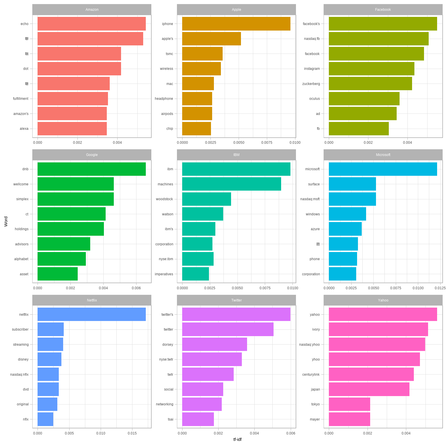
图 5.5: The 8 words with the highest tf-idf in recent articles specific to each company
If we were interested in using recent news to analyze the market and make investment decisions, we’d likely want to use sentiment analysis to determine whether the news coverage was positive or negative. Before we run such an analysis, we should look at what words would contribute the most to positive and negative sentiments, as was shown in Chapter 2.4. For example, we could examine this within the AFINN lexicon (Figure 5.6).
load("data/afinn.rda")
stock_tokens %>%
  anti_join(stop_words, by = "word") %>%
  count(word, id, sort = TRUE) %>%
  inner_join(afinn, by = "word") %>%
  group_by(word) %>%
  summarize(contribution = sum(n * value)) %>%
  top_n(12, abs(contribution)) %>%
  mutate(word = reorder(word, contribution)) %>%
  ggplot(aes(word, contribution)) +
  geom_col() +
  coord_flip() +
  labs(y = "Frequency of word * AFINN value")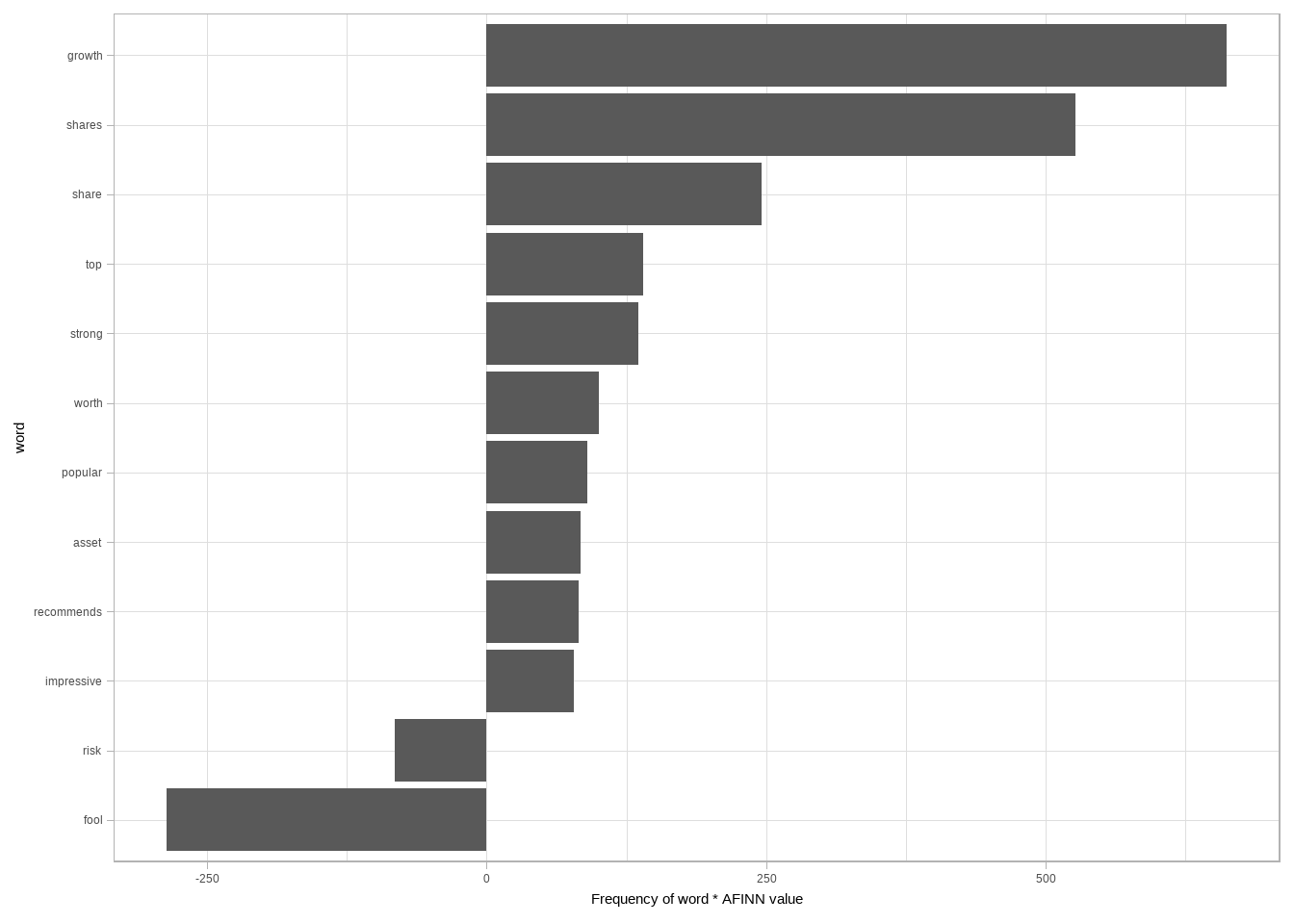
图 5.6: The words with the largest contribution to sentiment values in recent financial articles, according to the AFINN dictionary. The ‘contribution’ is the product of the word and the sentiment value.
In the context of these financial articles, there are a few big red flags here. The words “share” and “shares” are counted as positive verbs by the AFINN lexicon (“Alice will share her cake with Bob”), but they’re actually neutral nouns (“The stock price is $12 per share”) that could just as easily be in a positive sentence as a negative one. The word “fool” is even more deceptive: it refers to Motley Fool, a financial services company. In short, we can see that the AFINN sentiment lexicon is entirely unsuited to the context of financial data (as are the NRC and Bing lexicons).
Instead, we introduce another sentiment lexicon: the Loughran and McDonald dictionary of financial sentiment terms (Loughran and McDonald 2011). This dictionary was developed based on analyses of financial reports, and intentionally avoids words like “share” and “fool,” as well as subtler terms like “liability” and “risk” that may not have a negative meaning in a financial context.
The Loughran data divides words into six sentiments: “positive,” “negative,” “litigious,” “uncertain,” “constraining,” and “superfluous.” We could start by examining the most common words belonging to each sentiment within this text dataset.
load("data/loughran.rda")
stock_tokens %>%
  count(word) %>%
  inner_join(loughran, by = "word") %>%
  group_by(sentiment) %>%
  top_n(5, n) %>%
  ungroup() %>%
  mutate(word = reorder(word, n)) %>%
  ggplot(aes(word, n)) +
  geom_col() +
  coord_flip() +
  facet_wrap(~ sentiment, scales = "free") +
  ylab("Frequency of this word in the recent financial articles")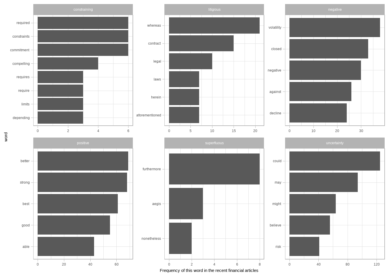
图 5.7: The most common words in the financial news articles associated with each of the six sentiments in the Loughran and McDonald lexicon
These assignments (Figure 5.7) of words to sentiments look more reasonable: common positive words include “strong” and “better,” but not “shares” or “growth,” while negative words include “volatility” but not “fool.” The other sentiments look reasonable as well: the most common “uncertainty” terms include “could” and “may.”
Now that we know we can trust the dictionary to approximate the articles’ sentiments, we can use our typical methods for counting the number of uses of each sentiment-associated word in each corpus.
stock_sentiment_count <- stock_tokens %>%
  inner_join(loughran, by = "word") %>%
  count(sentiment, company) %>%
  spread(sentiment, n, fill = 0)

stock_sentiment_count
## # A tibble: 9 x 7
## company constraining litigious negative positive superfluous uncertainty
## <chr> <dbl> <dbl> <dbl> <dbl> <dbl> <dbl>
## 1 Amazon 7 8 83 139 3 70
## 2 Apple 9 11 161 156 2 132
## 3 Facebook 3 32 128 143 4 81
## 4 Google 7 8 60 103 0 58
## 5 IBM 8 22 147 147 0 104
## 6 Microsoft 6 19 92 129 3 116
## 7 Netflix 3 7 111 161 0 106
## 8 Twitter 4 12 155 79 1 75
## 9 Yahoo 3 28 130 69 0 71It might be interesting to examine which company has the most news with “litigious” or “uncertain” terms. But the simplest measure, much as it was for most analysis in Chapter 2, is to see whether the news is more positive or negative. As a general quantitative measure of sentiment, we’ll use “(positive - negative) / (positive + negative)” (Figure 5.8).
stock_sentiment_count %>%
  mutate(value = (positive - negative) / (positive + negative)) %>%
  mutate(company = reorder(company, value)) %>%
  ggplot(aes(company, value, fill = value > 0)) +
  geom_col(show.legend = FALSE) +
  coord_flip() +
  labs(x = "Company",
       y = "Positivity value among 20 recent news articles")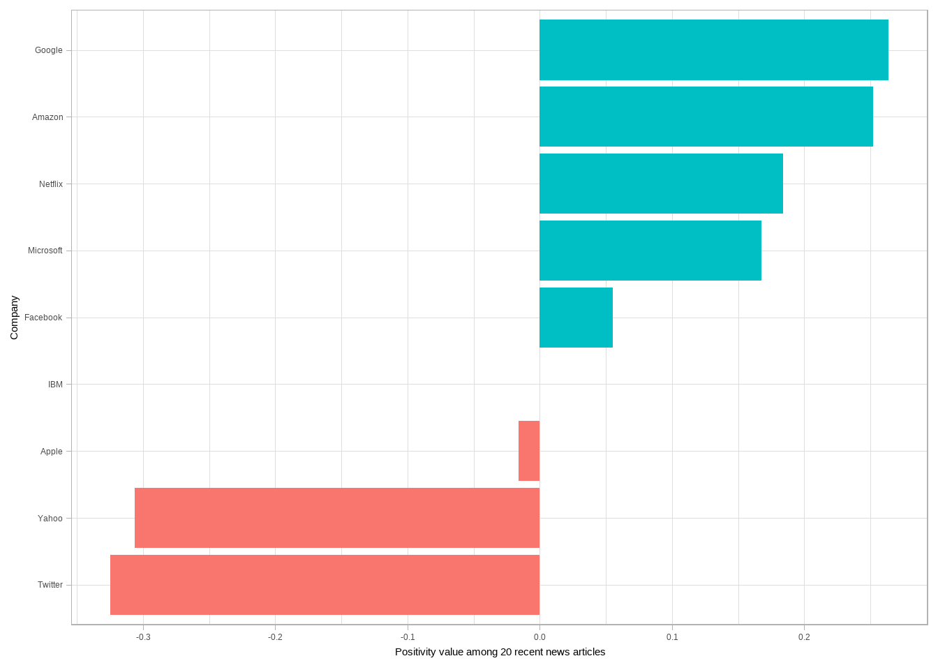
图 5.8: “Positivity” of the news coverage around each stock in January 2017, calculated as (positive - negative) / (positive + negative), based on uses of positive and negative words in 20 recent news articles about each company
Based on this analysis, we’d say that in January 2017 most of the coverage of Yahoo and Twitter was strongly negative, while coverage of Google and Amazon was the most positive. A glance at current financial headlines suggest that it’s on the right track. If you were interested in further analysis, you could use one of R’s many quantitative finance packages to compare these articles to recent stock prices and other metrics.
5.4 小结
Text analysis requires working with a variety of tools, many of which have inputs and outputs that aren’t in a tidy form. This chapter showed how to convert between a tidy text data frame and sparse document-term matrices, as well as how to tidy a Corpus object containing document metadata. The next chapter will demonstrate another notable example of a package, topicmodels, that requires a document-term matrix as input, showing that these conversion tools are an essential part of text analysis.